DataDependence

The class autonlu.data_dependence.DataDependence can be used to visualize the relationship between the amount of training data and the accuracy of the resulting model. This information can be used to determine whether labeling additional data is probably going to be useful or not.

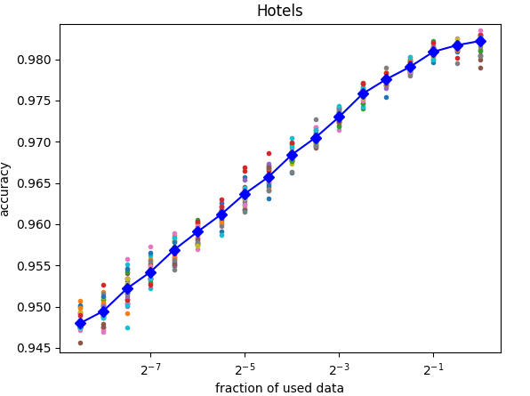
Here an example for a case where additional training data is likely not going to improve the resulting model (note that the x axis has a logarithmic scale):

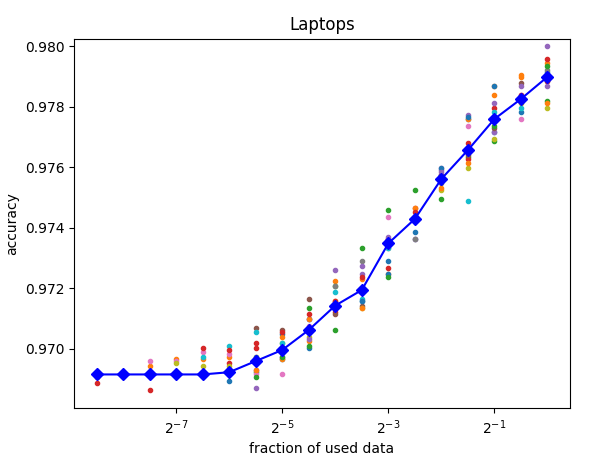
Here an example plot for a case where additional training data is probably going to improve the resulting model:

class autonlu.data_dependence.DataDependence(model_folder, device=None)

This class helps to estimate the accuracy of a model in dependence of the amount of training data. To this end, the function DataDependence.train_smaller_models() trains many models on subsets of the full training data. Since this is quite time consuming, a faster OMI-model is used.

Parameters

• model_folder (str) –

  A path or name of the model that should be used. Will be sent through autonlu.get_model_dir() and can therefore be:

  • The path to a model

  • The name of a model available in Studio

  • The name of a model available in the Huggingface model repo

• device (Optional[str]) –

  Which device the model should be used on ("cpu" or "cuda"). If None, a device will be automatically selected:

  If a CUDA capable GPU is available, it will automatically be used, otherwise the cpu. This behaviour can be overwritten by specifically setting the environment variable DO_DEVICE to either "cpu" or "cuda". autonlu.utils.get_best_device() is used to select the device.

Example

>>> # Load/get datasets and label Xtrain, Ytrain, Xvalid, Yvalid, Xtest, Ytest
>>> data_dependence = DataDependence("bert-base-uncased", "cuda")
>>> data_dependence.train_smaller_models(Xtrain, Ytrain, Xvalid, Yvalid, Xtest, Ytest,
                                         save_file="my_resuts.p", plot_file="my_plot.png")

train_smaller_models(X, Y, valX, valY, testX, testY, nb_datapoints=20, growth_factor=1.4142135623730951, nb_iterations=1, recycle_smaller_model=False, nb_opti_steps=70000, save_file=None, plot_file=None, plot_title=None, verbose=True)

For a given dataset, several sub-datset consisting of different fractions of the main dataset are used to train the basemodel. At the end, the accuracy of the different models can be saved and/or plotted.

Parameters

• X (List[Union[str, Tuple[str, str]]]) – Input samples. Either a list of strings for text classification or a list of pairs of strings for text pair classification.

• Y (List[str]) – Training target. List containing the correct labels as strings.

• valX (List[Union[str, Tuple[str, str]]]) – Input samples used for validation of the model during training.

• valY (List[str]) – Training target used for validation of the model during training.

• testX (List[Union[str, Tuple[str, str]]]) – Input samples used for calculating final results

• testX – Targets used for calculating final results

• nb_datapoints (int) – determines the number of dataset fractions.

• growth_factor (float) –

  determines the size-factor between different datasets. Example: For nb_datapoints = 5 and growth_factor = 2, sub-datasets are

  downscaled by the factors 1/16; 1/8; 1/4; 1/2; 1

  For groth_factor = 1 or growth_factor = 0, a linear scaling is assumed. Example: For nb_datapoints = 5 and growth_factor = 0 (1), sub-datasets are

  downscaled by the factors 1/5; 1/4; 1/3; 1/2; 1

• nb_iterations (int) – The number of repetitions (with newly mixed datasets)

• recycle_smaller_model (bool) – After a model was trained on a smaller dataset, the trained model might be used as initial model for the next bigger dataset. Choose True tohave the model recycled and False to start each time with a fresh model.

• nb_opti_steps (int) – This number correlates with the maximal number of optimization steps. Since the relation is non linear, one shouldn’t take the exact number to seriously. However, reducing nb_opti_steps makes optimization faster, increasing makes it more precise.

• save_file (Optional[str]) – A file path, where to save the results (pickled)

• plot_file (Optional[str]) – A file path, where a plot of the results will be saved each iteration (older ones are overwritten). Hence, you might already check preliminary results before the program has finished.

• plot_title (Optional[str]) – Title which appears in the figure.

• verbose (bool) – If True, information about the progress will be shown on the terminal.